Introduction
Fluorescence Lifetime Imaging Microscopy (FLIM) goes beyond fluorescence intensity measurements to image the time-dependent properties of a sample. This technique is highly sensitive to changes in the microenvironment of the fluorophore, making it valuable for high-quality biological imaging of plant and animal tissue.
FLIM measures the spatial variation of a fluorophore’s fluorescence lifetime, providing richer data than traditional intensity-based methods like widefield fluorescence. FLIM is advantageous over fluorescence intensity because it is independent of concentration, sample thickness, and photobleaching, and can provide more detailed information pertaining to environmental factors such as oxygen content and pH.
Beyond biology, FLIM is increasingly used to study materials like nanomaterials, solar panels and semiconductors. FLIM can measure the spatial variation in charge carrier lifetimes across semiconductor materials and investigate loss mechanisms.
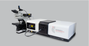
This Application Note demonstrates FLIM of plant tissue using MicroPL upgrade to the Edinburgh Instruments FS5 and FLS1000 photoluminescence (PL) spectrometers (Figure 1). The technique revealed the intricate structure and variations in the local microenvironment across a section of convallaria rhizome tissue.

Figure 1. MicroPL coupled to an FS5 Spectrofluorometer and FLS1000 PL Spectrometer for FLIM mapping.
The sample presented in this Application Note is a section of convallaria rhizome, also known as lily of the valley, stained with acridine orange. FLIM mapping was performed using the MicroPL coupled to an FS5 Spectrofluorometer (Figure 2).

Figure 2. Example experimental setup for FLIM by coupling the MicroPL to an FS5 Spectrofluorometer.
An EPL-485 pulsed laser source was directly coupled to the MicroPL, and measurements were collected using Time-Correlated Single Photon Counting (TCSPC). Full experimental parameters are shown in Table 1.
Table 1. Experimental parameters of FLIM mapping
| Parameter | Measurement |
|---|---|
| Excitation Source | EPL-485 |
| Acquisition Mode | TCSPC |
| Dichoric Filters | 495 nm |
| Objective Lens | 40x |
| Emission Wavelength | 540 nm |
| Emission Bandwidth | 3 nm |
| Map Step Size | 1 µm |
| Repetition Rate | 20 MHz |
| Dwell Time | 0.3 s |
| Detector | Photomultiplier Tube |
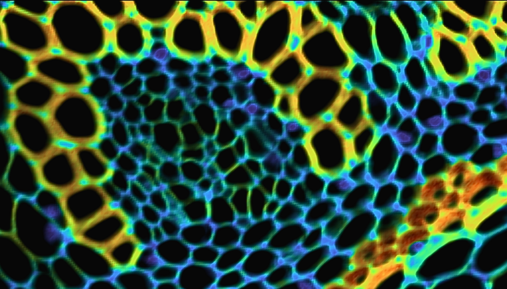
A FLIM map of the convallaria tissue was collected and is shown in Figure 3. The decays were fitted using a two-component exponential and the false-coloured image is scaled to the amplitude average PL lifetime (<τ>a) in nanoseconds. The FLIM map reveals variation in lifetime across the lignified and pectin rich cell walls and allows visualisation of the concentric vascular bundles in the tissue.

Figure 3. FLIM image of convallaria rhizome stained with acridine orange. The acridine orange was excited at 20 MHz repetition rate using the EPL-485 laser source.
PL decays from two distinct regions were extracted and a comparison of the PL lifetime is shown in (Figure 4). The first point of interest (Point 1) was false-coloured blue on the FLIM map. This region had an amplitude average lifetime of 0.61 ns. In contrast, the second point of interest (Point 2), which was false-coloured orange on the FLIM map, had an amplitude average lifetime of 2.11 ns. These significant differences in fluorescence lifetime reveal different microenvironments for the fluorophore across the tissue.

Figure 4. Fluorescence decays from two different regions of FLIM image.
The MicroPL upgrade equips the FS5 or FLS1000 PL spectrometers for FLIM. FLIM can reveal spatial variations within a sample, offering insights into its microenvironment. This was demonstrated by using FLIM to reveal the intricate structure of Convallaria rhizome tissue. Overall, FLIM enables micro-scale analysis of diverse samples, from biological tissue to advanced materials like solar panels and semiconductors.