What is an Excitation Emission Matrix (EEM)?
An excitation emission matrix or EEM is quickly becoming a widely used measurement in the field of fluorescence spectroscopy. An EEM is a 3D scan that results in a contour plot of excitation wavelength versus emission wavelength versus fluorescence intensity. An example is shown in Figure 1.1, 2
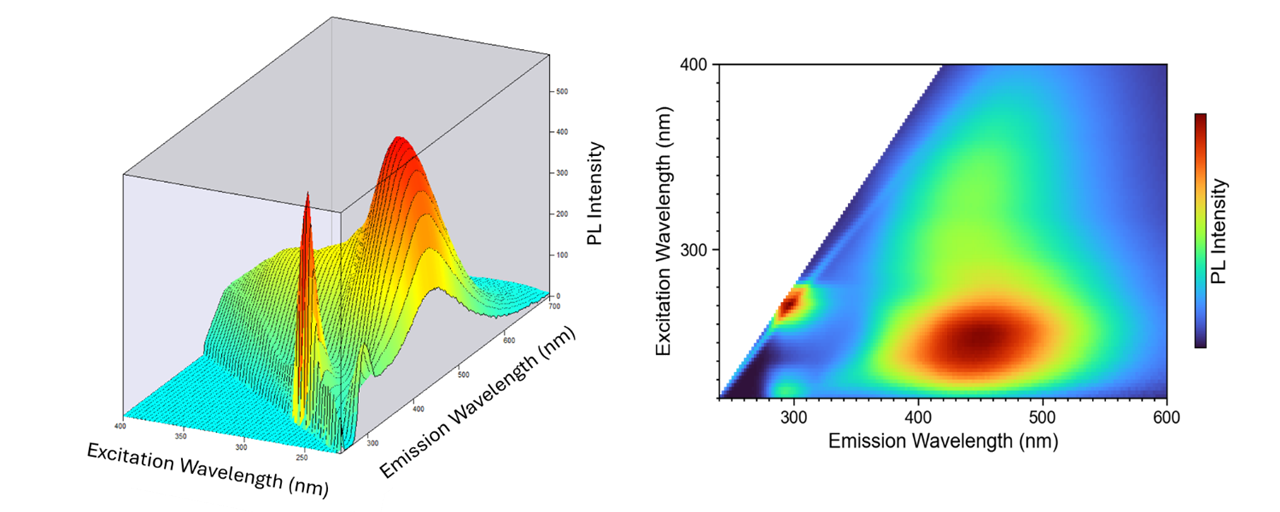
Figure 1. EEM of river water. Measurements were taken on an FLS1000 photoluminescence (PL) spectrometer.
EEM provides a detailed quantitative profile of a sample’s fluorescence, often referred to as its molecular fingerprint. Because EEM captures a broad picture of a sample’s fluorescence in a single acquisition, it allows for fast and straightforward analysis of complex spectra, particularly those from multicomponent samples.
EEM was first introduced by Gregorio Weber in 1961 with the rationale that a sample exhibits excitation and emission spectra unique to a specific mixture of fluorophores present.3 In Weber’s earlier work, the goal was to determine the number of fluorophores in mixtures by varying the excitation and emission wavelengths and constructing a matrix of the resulting fluorescence intensities. The development of computer-controlled instrumentation and data analysis has enabled Weber’s matrix approach to become a standard analytical technique, known as EEM. EEMs are now used to identify very low concentrations of substances present in a sample.
EEM maps can be measured either by a series of emission scans with a stepwise increase or decrease of the excitation wavelength or by a series of synchronous scans with a stepwise increase of the excitation-emission offset.
A common feature of all EEMs is the presence of Rayleigh and Raman scatter bands. These do not represent the samples fluorescent fingerprint. These so-called scatter bands are visually easily identifiable and appear diagonally in the EEM as shown in Figure 2.
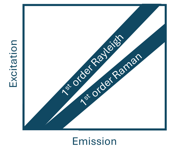
Figure 2. Rayleigh and Raman scattering in EEMs.
Rayleigh scattering is elastic scattering meaning that the photons scatter without a loss of energy and therefore Rayleigh scattering always appears at the same wavelength as the excitation light. In contrast, Raman scattering is inelastic scattering. During this scattering, energy is transferred between scattered photon and molecule, resulting in the scattering occurs at a different wavelength to the excitation source.
EEMs contain a large amount of data which can hinder the ability to use all the information collected. To fully understand fluorescence EEM, multivariate analysis may be required. This can include techniques such as classical least squared (CLS), principal component analysis (PCA) and parallel factor analysis (PARAFAC). As scattering occurs across the whole EEM it is important to remove such artifacts prior to data analysis.
The inner filter effect (IFE) is a common obstacle in fluorescence spectroscopy, particularly for EEM measurements. The IFE can be divided into primary and secondary effects, shown in Figure 3.1, 4
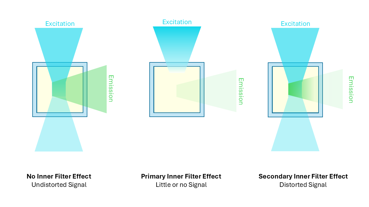
Figure 3. Fluorescence inner filter effect (IFE). Primary versus secondary IFE.
The primary IFE occurs when a sample is very concentrated, and the excitation beam is attenuated by the sample so only the surface of the cuvette fluoresces. The centre of the cuvette, which is at the focal point of the emission monochromator, has low excitation intensity and therefore weak fluorescence emission.
The secondary IFE describes when the excitation and emission spectra overlap significantly. This leads to the light emitted at the centre of the cuvette being reabsorbed by the sample itself before being emitted towards the detector.
Overall, the IFE causes spectral distortion and loss of signal. To avoid the IFE, the sample must be diluted, typically to an absorbance less than 0.1. Alternatively, a mathematical correction can be applied. The correction is most often based on the measured absorbance of the sample.
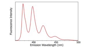
EEM measurements are useful in the application of food analysis. This is because this technique can investigate complex mixtures of ingredients in a food product. An example of how this is the study of a fizzy drink as shown in Figure 4.
Figure 4. Contour EEM 3D plot of a fizzy drink. Measurements taken on FS5 Spectrofluorometer.
The 3D plot can be displayed as a heatmap of excitation vs emission vs fluorescence intensity. Emission and excitation spectra can be visualised at different points from the heatmap (Figure 5).
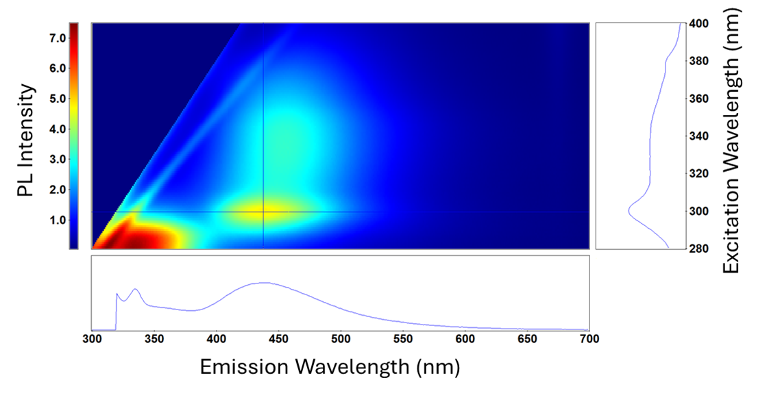
Figure 5. EEM heatmap of a fizzy drink. Measurements taken on FS5 Spectrofluorometer.
This data is analsyed to determine the quality and composition of this fizzy drink sample. This could include investigating the additive, colourants and nutritional ingredients of the product.
The most common applications of EEM are in food and water quality analysis. In the food industry, EEM can be used to determine the, quality, and geographic origin of food products. For example, EEM can help verify the authenticity and origin of foods like tea, oil, wine, and honey, as well as assess their quality. For example, EEM can differentiate between olive oils with distinctive flavour characteristics by analysing their unique fluorescence signatures.5
EEM is also used for detecting and monitoring dissolved organic material (DOM) in water, including in freshwater ecosystems, drinking water sources, and wastewater treatment plants. This includes detecting components such as amino acids, fulvic acid, humic acid, and other decomposition products in natural water sources (Figure 6). Detection of DOMs, along with disinfection by-products, is vital for monitoring water treatment processes. For instance, EEM can help detect the presence of specific organic compounds that might react with disinfectants to form harmful byproducts.

Figure 6. EEM heatmap of river water for studying dissolved material present in water sources.